# APR Pipeline Since 2009  ---

Let me start the talk by asking this question.

The answer is definitely yes if we compare the results we got with jGenProg and one of the recent APR tools, SRepair.

In other words, do APR techniques explore the patch space efficiently?

To answer the question, let's briefly review the typical APR pipeline. Given a buggy program and a test suite, we first obtain fault localization information. Then, based on that information, we repeat to generate and validate patch candidates. Here, the order of generating patch candidates is determined by a patch scheduling algorithm.

Most APR tools use a very simple patch scheduling algorithm. It basically visits each program location and generates N patch candidates at that location.

This is a rather crude algorithm. Spectrum-based fault localization is often used in APR, and it is well-known that multiple locations often have the same suspiciousness score.

As a result, a large number of patch candidates share the same rank. And of course, there is no guarantee that any of the these rank 1 patch passes all tests.

In fact, the patch scheduling algorithm of the early days of APR research was more sophisticated, as you are well aware.

Roughly speaking, the statement to be mutated is chosen at random in proportion to the suspiciousness score of the statement.

However, as will be shown in our experimental results, GenProg's patch scheduling algorithm does not always perform better than the simple algorithm mentioned before.

We drew inspiration from fuzzing, whose success is largely attributed to its high efficiency.

The problem of fuzzing is basically to search for a bug-revealing input from the input space. To perform a search efficiently, many fuzzing algorithms use an online stochastic scheduling algorithm. This is in contrast to APR where offline deterministic scheduling algorithm is mostly used as explained earlier.

To perform an online search, many fuzzers use a concept of interesting input. Simply speaking, an interesting input is an input that covers a new execution path. Once an interesting input is found, it is further mutated to find a bug-revealing input or another interesting input.

So, fuzzing can be viewed as a process of searching for interesting inputs.

# APR  - Search space = Patch space ---

In APR, we have a correct patch and a plausible patch.

In the old days, a plausible patch was considered bad. Early APR tools stopped searching for a patch once a plausible patch was found, thereby loosing the chance to find a correct one.

However, there is no guarantee that a first-found plausible patch is correct. To avoid this problem, many recent APR tools generate multiple plausible patches.

For example, VarFix generates a ranked list of plausible patches.

Similar approaches are taken in other tools such as CPR. In the case of CPR, once a pool of plausible patches is found, invalid patches are filtered out using concolic execution.

We also proposed a semi-automatic method to filter out incorrect plausible patches. Our approach allows the user to specify a condition under which the patched version should behave identically to the original version.

So, if we use such a pipeline that generates multiple patches, APR can be viewed as a process of searching for plausible patches, followed by selecting a correct patch among them.

In this talk, I will focus on the first phase.

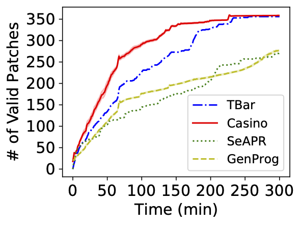
To give you a clearer picture of our work, let me first show you the results of our approach.

Our patch scheduling algorithm is generic and can be applied to many different APR tools. We applied our algorithm named Casino to six APR tools, including TBar, AlphaRepair, and Recoder.

Each plot shows how many plausible patches are found over time in each APR tool. The blue curve shows the performance of the original tool, and the red curve shows the performance after applying our algorithm. In all three tools, the red curve grows faster than the blue curve, indicating the better efficiency of our algorithm.

We have also further improved the efficiency of our algorithm. In each plot, the blue curve again shows the performance of the original tool, and the green curve shows the performance of our first algorithm, Casino. Lastly, the red curve shows the performance of our improved algorithm, Gresino. Clearly, Gresino outperforms both Casino and the original tool.

Now I will explain how our first algorithm works. To explore the patch space efficiently, we view the patch space as a tree structure. Then, selecting a patch candidate amounts to navigating this tree. At each layer of the tree, we choose a file to modify, a method to modify, and a location to modify. Once a patch location is chosen, we choose a patch candidate at that location at random in a way that I will explain later.

How do we navigate the tree efficiently?

A short answer is that we view the patch scheduling problem as a multi-armed bandit problem.

Our situation can be specifically modeled as a Bernoulli bandit problem. We need to speculate the probability of success of each arm. And each arm can have a different probability of success.

The Bernoulli bandit problem can be solved by the Thompson sampling algorithm that works in the following three steps. First, for each arm $k$, we sample $\theta_k$ from its distribution. Let's say we are about to choose between method 1 and method 2. Let's assume that the left arm is associated with this Beta distribution and the right arm is associated with that Beta distribution. It is likely that a higher value is sample from the right arm, in which case we choose the right arm. However, note that Thompson sampling still allows to choose the left arm with a smaller probability.

- Distribution of $\theta_k$: Beta distribution $(\alpha_k, \beta_k)$ | $Beta(\alpha=2,\beta=2)$ | $Beta(\alpha=3,\beta=2)$ | $Beta(\alpha=5,\beta=2)$ | | --- | --- | --- | |  |  |  |

What if we find an interesting patch? Then, we update the distributions of the corresponding edges. For example, if this was the distribution of this edge before the update, its right-hand side one shows the distribution after the update. Notice that the distribution after the update is more left skewed, indicating that selecting this edge looks more promising than before.

# Evaluation  - GenProg$^{SL}$: modifies a single location - Choose a program location $l$ at random proportional to the suspicious score of $l$ - Among the patch candidates available at $l$, choose one at random ---

Then the natural question that arises is: Can we invent a grey-box approach that performs better than the black-box approach?

Each edge is associated with critical branches. These critical branches are obtained after executing interesting patches observed in the corresponding subtree. Unlike in the black-box approach, we assign a beta distribution to each critical branch.