CSE411: Introduction to Compilers

Interval Analysis

Jooyong Yi (UNIST)

Example

#include <stdio.h>
int main(int argc, char **argv) {
  char buf[8];         // buffer for eight characters
  gets(buf);           // read from stdio (sensitive function!)
  printf("%s\n", buf); // print out data stored in buf
  return 0;            // 0 as return value
}

Buffer Overflow

            |             |             |              |
---------------------------             ----------------
            | Parameters  |             | parameters   |
   frame    | return addr |    ---->    | function ptr |
            | buf[4...7]  |             | buf[4..7]    |
            | buf[0...3]  |             | buf[0..3]    |
---------------------------             ----------------
            |             |             |              |

Wishful Thinking

#include <stdio.h>
int main(int argc, char **argv) {
  char buf[8];         // buffer for eight characters
  gets(buf);           // read from stdio (sensitive function!)
  printf("%s\n", buf); // print out data stored in buf
  return 0;            // 0 as return value
}

• What if a compiler can detect buffer overflow?

Simple Buffer Overflow Analysis

   _________________________
   | 0 | 1 | 2 | 3 | 4 | 5 |
   ‾‾‾‾‾‾‾‾‾‾‾‾‾‾‾‾‾‾‾‾‾‾‾‾‾
   ↑
   buf

• Is buf[i] safe?

Simple Buffer Overflow Analysis

   _________________________
   | 0 | 1 | 2 | 3 | 4 | 5 |
   ‾‾‾‾‾‾‾‾‾‾‾‾‾‾‾‾‾‾‾‾‾‾‾‾‾
   ↑
   buf

• Is buf[i] safe?
  • Is 0 <= i < 6?

Interval Analysis

            1: x = 0; y = 0
               ↓   
            2: x < z  
               |
   ----------------------- 
   ↓                     ↓
  3: x = x + 1        4: x = x + 2
   |                     |
   -----------------------
               ↓
          5: y = x + x
               ↓
          6: w = buf[y]                                                               

• Dataflow values?
• Transfer function?
• Join function?

Interval Analysis

            1: x = 0; y = 0
               ↓   
            2: x < z  
               |
   ----------------------- 
   ↓                     ↓
  3: x = x + 1        4: x = x + 2
   |                     |
   -----------------------
               ↓
          5: y = x + x
               ↓
          6: w = buf[y]                                                               

• Dataflow values
  • For each variable, an interval [l, u]
    • l: the lower bound
    • u is the upper bound

Interval Analysis

            1: x = 0; y = 0
               ↓   
            2: x < z  
               |
   ----------------------- 
   ↓                     ↓
  3: x = x + 1        4: x = x + 2
   | x: [1,1]            | x: [2,2]
   -----------------------
               ↓ x: [?,?]
          5: y = x + x
               ↓
          6: w = buf[y]                                                               

• Transfer function?
• Join function?

Interval Analysis

            1: x = 0; y = 0
               ↓   
            2: x < z  
               |
   ----------------------- 
   ↓                     ↓
  3: x = x + 1        4: x = x + 2
   | x: [1,1]            | x: [2,2]
   -----------------------
               ↓ x: [1,2]
          5: y = x + x
               ↓ y: [?,?]
          6: w = buf[y]                                                               

• Transfer function?
• Join function?

Interval Analysis

            1: x = 0; y = 0
               ↓   
            2: x < z  
               |
   ----------------------- 
   ↓                     ↓
  3: x = x + 1        4: x = x + 2
   | x: [1,1]            | x: [2,2]
   -----------------------
               ↓ x: [1,2]
          5: y = x + x
               ↓ y: [2,4]
          6: w = buf[y]                                                               

• Transfer function?
• Join function?

Interval Analysis

            1: x = 0; y = 0
               ↓   
            2: x < z  
               |
   ----------------------- 
   ↓                     ↓
  3: x = x + 1        4: x = x + 2
   | x: [1,1]            | x: [2,2]
   -----------------------
               ↓ x: [1,2]
          5: y = x + x
               ↓ y: [2,4]
          6: w = buf[y]                                                               

• Transfer function

Interval Analysis

            1: x = 0; y = 0
               ↓   
            2: x < z  
               |
   ----------------------- 
   ↓                     ↓
  3: x = x + 1        4: x = x + 2
   | x: [1,1]            | x: [2,2]
   -----------------------
               ↓ x: [1,2]
          5: y = x + x
               ↓ y: [2,4]
          6: w = buf[y]                                                               

• Join function
  • Forward or backward?
  • May or must?

Interval Analysis

            1: x = 0; y = 0
               ↓   
            2: x < z  
               |
   ----------------------- 
   ↓                     ↓
  3: x = x + 1        4: x = x + 2
   | x: [1,1]            | x: [2,2]
   -----------------------
               ↓ x: [1,2]
          5: y = x + x
               ↓ y: [2,4]
          6: w = buf[y]                                                               

• Join function
  • OUT[B] = IN[S] ?

Reaching Definition Analysis

  B0: y < N  -----------------------------       
        ↓                                ↓
  B1: x = 1                       B3: x = 0
        ↓   RD(x) = {B1, B3}             |
  B2: y = x + 1  <------------------------

• OUT[B] = IN[S]

                       {B1,B3}
                       /     \
                    {B1}     {B3} 
                       \     /
                          ∅

Lattice

                       {B1,B3}
                       /     \
                    {B1}     {B3} 
                       \     /
                          ∅

• ∅ ⊂ {B1}, ∅ ⊂ {B3}
• {B1} ⊂ {B1, B3}, {B3} ⊂ {B1, B3}
• {B1} ∪ {B3} = {B1,B3}

Lattice

                          E4
                       /      \
                      E2      E3
                       \      /
                          E1

• E1 ⊏ E2, E1 ⊏ E3
• E2 ⊏ E4, E3 ⊏ E4
• E2 ∪ E3 = E4

Lattice

            1: x = 0; y = 0
               ↓   
            2: x < z  
               |
   ----------------------- 
   ↓                     ↓
  3: x = x + 1        4: x = x + 2
   | x: [1,1]            | x: [2,2]
   -----------------------
               ↓ x: [1,2]
          5: y = x + x
               ↓ y: [2,4]
          6: w = buf[y]                                                               

             [1,2]
           /      \
        [1,1]     [2,2]

• [1,1] ⊏ [1,2], [2,2] ⊏ [1,2]
• [1,1] ⨆ [2,2] = [1,2]

Interval Analysis

            1: x = 0; y = 0
               ↓   
            2: x < z  
               |
   ----------------------- 
   ↓                     ↓
  3: x = x + 1        4: x = x + 2
   | x: [1,1]            | x: [2,2]
   -----------------------
               ↓ x: [1,2]
          5: y = x + x
               ↓ y: [2,4]
          6: w = buf[y]                                                               

• Join function
  • OUT[B] = IN[S]

Lattice

• A lattice is a partially ordered set where x ⊔ y and x ⊓ y exist for all x,y ∈

                         E4
                       /    \
                      E2    E3
                       \    /
                         E1

• Join operation: E2 ⊔ E3 = E4
• Meet operation: E2 ⊓ E3 = E1

Partially Ordered Set (Poset)

• A poset is where is a set and ⊑ is a binary relation for the elements of that satisfies the following properties:
  • Reflexive:
  • Antisymmetric: if and , then
  • Transitive: if and , then

Poset ({∅, {B1}, {B3}, {B1,B3}}, ⊆)

                       {B1,B3}
                       /     \
                    {B1}     {B3} 
                       \     /
                          ∅

Lattice and Reaching Definition Analysis

  B0: y < N  -----------------------------       
        ↓                                ↓
  B1: x = 1                       B3: x = 0
        ↓   RD(x) = {B1, B3}             |
  B2: y = x + 1  <------------------------                                                   

• OUT[B] = IN[S]

                       {B1,B3}
                       /     \
                    {B1}     {B3} 
                       \     /
                          ∅                                                                   

• At each node of the control flow graph, we maintain a dataflow value:
  • Initially, ∅
  • Keep updating until reaching a fixed point
  • Always move to a higher level in the lattice

Reaching Definition Analysis Example

• IN[B] = OUT[P]
• OUT[B] = (IN[B] - kill[B]) gen[B]
  • : the set of predecessors of B.

          1: a = 5                                                            Iteration 1         Iteration 2         Iteration 3
             ↓                                 |  n  |  gen(n) | kill(n) |  IN[n]  |  OUT[n] |  IN[n]  |  OUT[n] |  IN[n]  |  OUT[n] |
          2: c = 1                             |:---:|:-------:|:-------:|:-------:|:-------:|:-------:|:-------:|:-------:|:-------:|
          ↓                                    |  1  |   {1}   |   {5}   |    ∅    |   {1}   |    ∅    |   {1}   |    ∅    |   {1}   |
  ----->  3: c > a  -------------              |  2  |   {2}   |  {4,6}  |   {1}   |  {1,2}  |   {1}   |  {1,2}  |   {1}   |  {1,2}  |
  |       ↓                     |              |  3  |    ∅    |    ∅    |  {1,2}  |  {1,2}  | {1,2,4} | {1,2,4} | {1,2,4} | {1,2,4} | 
  |       4: c = c + c          ↓              |  4  |   {4}   |  {2,6}  |  {1,2}  |  {1,4}  | {1,2,4} |  {1,4}  | {1,2,4} |  {1,4}  |  
  |-------|                 5: a = c - a       |  5  |   {5}   |   {1}   |  {1,2}  |  {2,5}  | {1,2,4} | {2,4,5} | {1,2,4} | {2,4,5} |  
                                ↓              |  6  |   {6}   |  {2,4}  |  {2,5}  |  {5,6}  | {2,4,5} |  {5,6}  | {2,4,5} |  {5,6}  |  
                            6: c = 0

Lattice and May Analysis

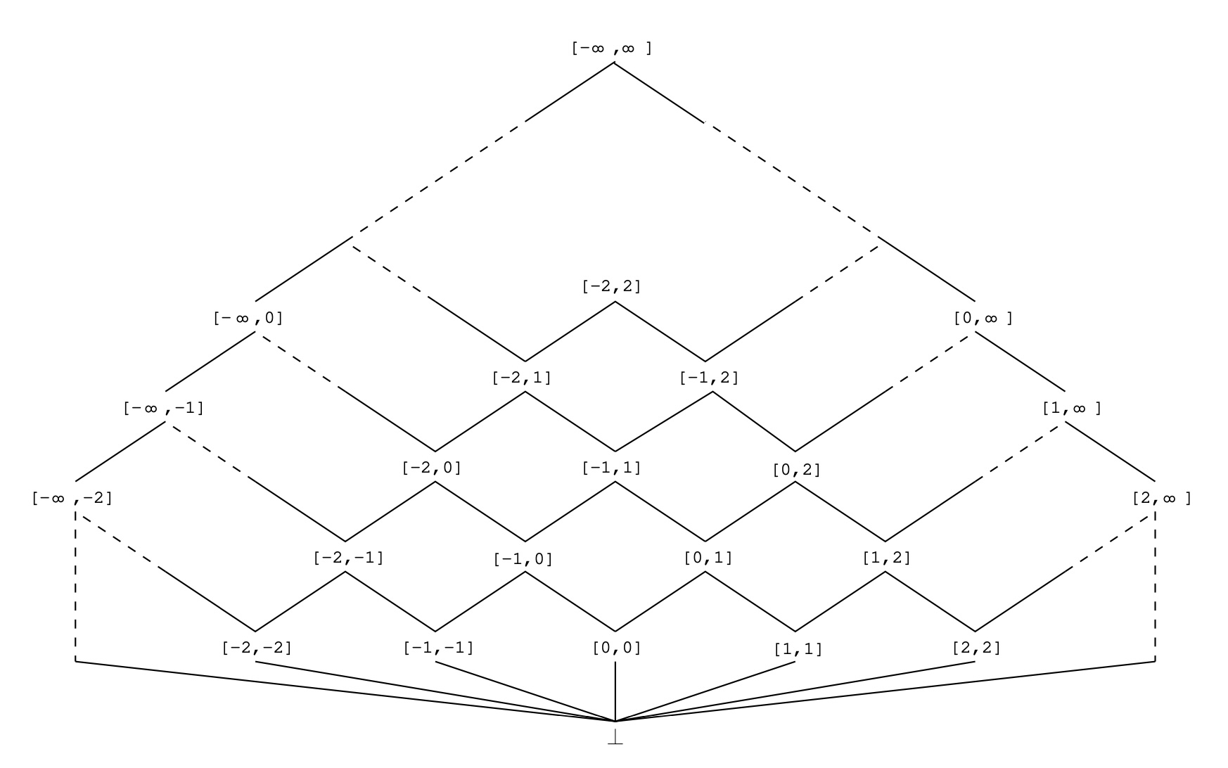
• Initially, the bottom (⊥)
• Keep updating until reaching a fixed point
• Always move to a higher level in the lattice

Lattice and May Analysis

• Initially, the bottom (⊥)
• Keep updating until reaching a fixed point
• Always move to a higher level in the lattice
  • Thus, a fixed point will be reached as long as the height of the lattice is finite

The Lattice for Interval Analysis