In this talk, I am going to introduce a new fuzzing concept called lightgrey-box fuzzing.

What is lightgrey-box fuzzing? Well, before introducing something new, let's start with something we are already familiar with. White-box fuzzing, grey-box fuzzing, and black-box fuzzing. How do they differ from each other? The differences between them could be explained in many different ways, and here is one of them.

White-box fuzzing generates inputs systematically by manipulating path conditions. Meanwhile, black-box fuzzing rapidly and often blindly produces random inputs. Grey-box fuzzing, sitting between the two, focuses the fuzzing effort on "interesting" inputs.

Generally speaking, the quality of inputs tends to be higher as the fuzzing approach is "whiter", whereas

the throughput of inputs tends to be larger as the fuzzing approach is "darker".

This contrast between input quality and throughput positions the grey-box fuzzing as the Goldilocks approach, as you are very well aware of. However, don't forget the three bears in the Goldilocks story.

Why should Goldilocks share a bed with a bear? She does not have to. She can have her own bed, in this case, the lightgrey-box fuzzing.

Jokes apart, we have two main goals with the lightgrey-box fuzzing. First, we want to generate high-quality input by using path conditions. Second, we want to achieve high throughput by using native execution.

Our key idea is simple. We inductively synthesize path conditions. Suppose we have two different sets of inputs whose native execution paths deviate at branch b1. Then, we pass these two sets of inputs to an inductive synthesizer to infer the condition of b1.

This idea can naturally be extended to synthesize path conditions inductively. Then, it is possible to generate inputs using these synthesized path conditions. I will explain soon how we use these path conditions to explore diverse execution paths.

Let me first show you a snippet of the results. We applied our lightgrey-box fuzzing named PathFinder to a well-known deep learning library, PyTorch. These plots show how branch coverage increases over time. Clearly, our approach overwhelmingly outperforms the existing SOTA tools using various approaches.

Among the compared SOTA tools, ACETest uses a two-stage approach. At the offline stage, it extracts partial PCs based on the manually defined rules for DL library operations. And then, at the online stage, it generates inputs using the obtained PCs. In contrast, our PathFinder learns the path conditions on the fly while performing the fuzzing.

Path conditions our approach synthesizes are typically only approximate. However, there is still an overlap between the input space of the precise path conditions and the obtained inductive path conditions.

Moreover, as the exploration proceeds, the path conditions can become more precise since more data points for synthesis are available.

So far, I did not explain how inductive path conditions can be used for path exploration. One noteworthy thing is that the typical path exploration strategy of symbolic execution cannot be used. Symbolic execution tools typically select one of the conditions in a path condition and negates it to explore a new path.

In our approach, a branch condition can be synthesized only after both directions are explored. There is no point in negating a branch condition that was already explored.

In fact, to be more precise, we do not maintain path conditions. Instead, we maintain path condition prefixes. Suppose we have a branch b4 and only the else direction is explored. Then, our path condition prefix does not contain the condition of b4.

Then, how do inductive path condition prefixes help path exploration?

Among many possible strategies, our tool currently uses probably the simplest one. We randomly select a path condition prefix and generate an input that satisfies the selected prefix. By doing so, we attempt to explore the sub-tree corresponding to the selected prefix.

Other strategies are also possible. For example, instead of random selection, an under-explored sub-tree can be prioritized. Or, a sub-tree witnessing new paths frequently can be prioritized. I think these are all good future research directions.

Now suppose we pick pi1 and generate an input satisfying it, expecting to take b1 followed by b2. However, due to the imprecision of the synthesized path conditions, the actual execution may follow a different path, say b1 followed by not b2. In this case, the input we just used is a counter-example for the current condition of b2. So, we refine the condition of b2 with this counter-example.

One thing noteworthy is that even an unexpected path may lead to a new path. This is particularly true at the early stage of the fuzzing.

As mentioned, we applied our lightgrey-box fuzzing to DL library APIs. This work was done in collaboration with my colleague at my university, Mijung Kim. She has been working on DL library testing techniques such as DocTer, and I have been developing the idea of lightgrey-box fuzzing, which makes a good match.

--- # Testing DL Libraries (PyTorch and TensorFlow) - Good (easy) targets for Lightgrey-box Fuzzing - A small number of data types are shared across many APIs. - int, float, Tensor, ...

--- # Syntax-Guided Inductive Synthesis ``` Var → (* API parameters *) Const → 0 | 1 | 2 | ... Cond → Var = Const | Var = Var | ¬Cond ... ``` - For a parameter `p` of the `Tensor` type, we use the following variables for synthesis. - `p.dtype`, `p.rank`, `p.dim0`. `p.dim1`, ...

For the branch condition synthesis, we used a syntax-guided inductive synthesizer called Duet invented by Woosuk Lee. For the variable syntax construct, we use the parameters of the API under test. DL library APIs often use a Tensor data type. When synthesizing a branch condition, we allow the synthesizer to use the attributes of the Tensor such as dtype, rank, and dimensions.

We compare our tool, PathFinder, with five existing tools. Four of them were already shown in the previous slide. One remaining one is DeepREL. DeepREL is an extension of FreeFuzz where the main difference is that it reuses the test inputs obtained from one API to test another similar APIs. We did not use this orthogonal technique in our tool.

And these are results for TensorFlow. Again, our tool outperforms the existing tools. However, the coverage curves grow more slowly than in the PyTorch case. We conjecture that this is due to a large number of non-deterministic branches in TensorFlow. A TensorFlow API has on average 25 times more non-deterministic branches than a PyTorch API. Like in symbolic execution, non-deterministic branches hinder the effectiveness of lightgrey-box fuzzing.

So, we prune non-deterministic branches from the path conditions whenever detected.

These plots support our conjecture on the non-deterministic branches. The red dotted curve shows the coverage growth when non-deterministic branches are not pruned. The effect of the non-deterministic branch pruning is more pronounced in TensorFlow probably due to the larger number of non-deterministic branches. These plots also show the effectiveness of another optimization technique we used, staged synthesis.

Our staged synthesis strategy is to reduce the synthesis cost. Another important factor affecting the synthesis cost is condition refinement. Whenever refinement is performed, additional synthesis cost is incurred.

Recall that our goal is not in synthesizing the most precise path conditions. So, we do not refine path conditions that are already good enough. Specifically, we consider a branch condition good enough if its MCC score is greater than or equal to 0.6.

A large sample size can also increase the synthesis cost. So, we limit the sample size to 30.

Like in symbolic execution, we use an SMT solver to generate inputs. However, unlike in symbolic execution, we may pass the same PC prefix to the SMT solver multiple times. A problem is that an SMT solver tends to generate the same input for the same path condition prefix.

To address this issue, we strengthen a given path condition prefix with a random constraint.

So, is lightgrey-box fuzzing the Goldilocks technique? What do you think?

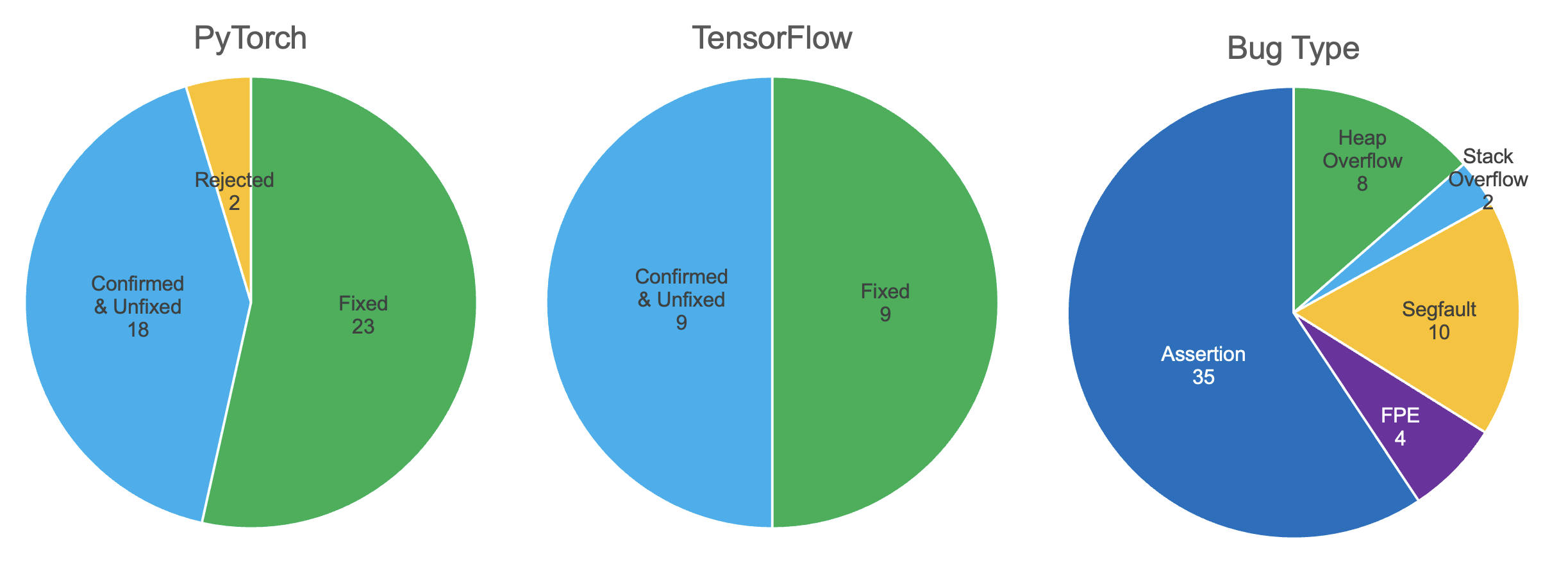
--- # Bug Finding